Lab 2: Multi Core Matrix Multiplication

Introduction

In Lab 1, you reviewed the standard matrix multiplication algorithm, implemented a tiled CPU version, and then mapped the same computation to a single Tensix core using TT-Metalium. In this lab, you will extend your matrix multiplication implementation from a single Tensix core to multiple cores by exploiting core-level parallelism. Then you will introduce a data reuse optimization that reduces traffic to device memory by keeping partial results in on-chip SRAM.

From Single Core to Multi Core Matrix Multiplication

The single-core TT-Metalium matmul implementation from Lab 1 created tiled tensors in the device DRAM and used two dataflow kernels to transfer data between the device DRAM and on-chip circular buffers, and a compute kernel to perform the matrix multiplication. In this lab, you will keep the same basic structure, but instead of running on a single core, you will:

• Create circular buffers and kernels on a set of cores.

• Divide the output tiles among those cores.

• Ensure that each core receives appropriate runtime arguments so that it processes the correct subset of output tiles.

Work Distribution for Multi Core Programs

The key idea in multi core programs is work distribution, where we break a large problem into smaller, ideally independent pieces and assign them to different cores to run in parallel. In a Single Program, Multiple Data (SPMD) computational model, each core executes the same code but operates on a different subset of the data. Achieving optimal performance generally requires keeping all cores busy (i.e., minimize idle time), and avoiding unnecessary communication.

Applying this principle to matrix multiplication, the computation itself is unchanged: we still multiply an MxK matrix A with a KxN matrix B to produce an MxN matrix C, and we still process data in tiles. However, instead of a single core computing all of C, the tiles of C are divided among multiple cores, and each core is responsible for computing a subset of those tiles in parallel with the others.

At a high level, the host code for multi core matrix multiplication needs to perform the following steps:

1. Determine the number of available (or desired) cores

   To distribute work among the cores, we need to know how many cores are available and how many of these cores we want to use. If the dataset is large enough and we only have one computational task, we may use all available cores. If we have multiple computational steps to perform, we may partition the work so that each step is performed on a subset of the cores.

2. Determine the amount of parallelizable work

   The amount of parallelizable work is specific to a given problem, and there may be multiple ways to partition the work. For the case of matrix multiplication, one way to partition the work is to observe that the computation is independent for each tile of the output matrix.

3. Partition work among cores

   If the amount of parallelizable work is larger than the number of cores, we need to split the work among the cores as evenly as possible. For matrix multiplication, each tile of the output takes the same amount of computation, so we can simply divide the number of tiles by the number of cores. In more complex cases, different parallelizable parts of the computation may require different amounts of work, so a more sophisticated method of splitting the work may be needed.

4. Configure each core

   For each core, we need to configure it to perform the correct subset of the work. While each core will execute the same code, the code usually needs to be parameterizable so each core can be configured to perform the correct subset of the work. For matrix multiplication, the parameters will include the output tiles that each core should process, and depending on exact implementation details, may also include the input tiles that each core should process.

Work Distribution in TT-Metalium

In this section, we describe TT-Metalium APIs for work distribution, and how they can be used to distribute work needed to perform matrix multiplication on multiple cores.

In the Tenstorrent architecture, the cores are organized into a 2D grid with each core uniquely identified by an index (x, y) in this grid.

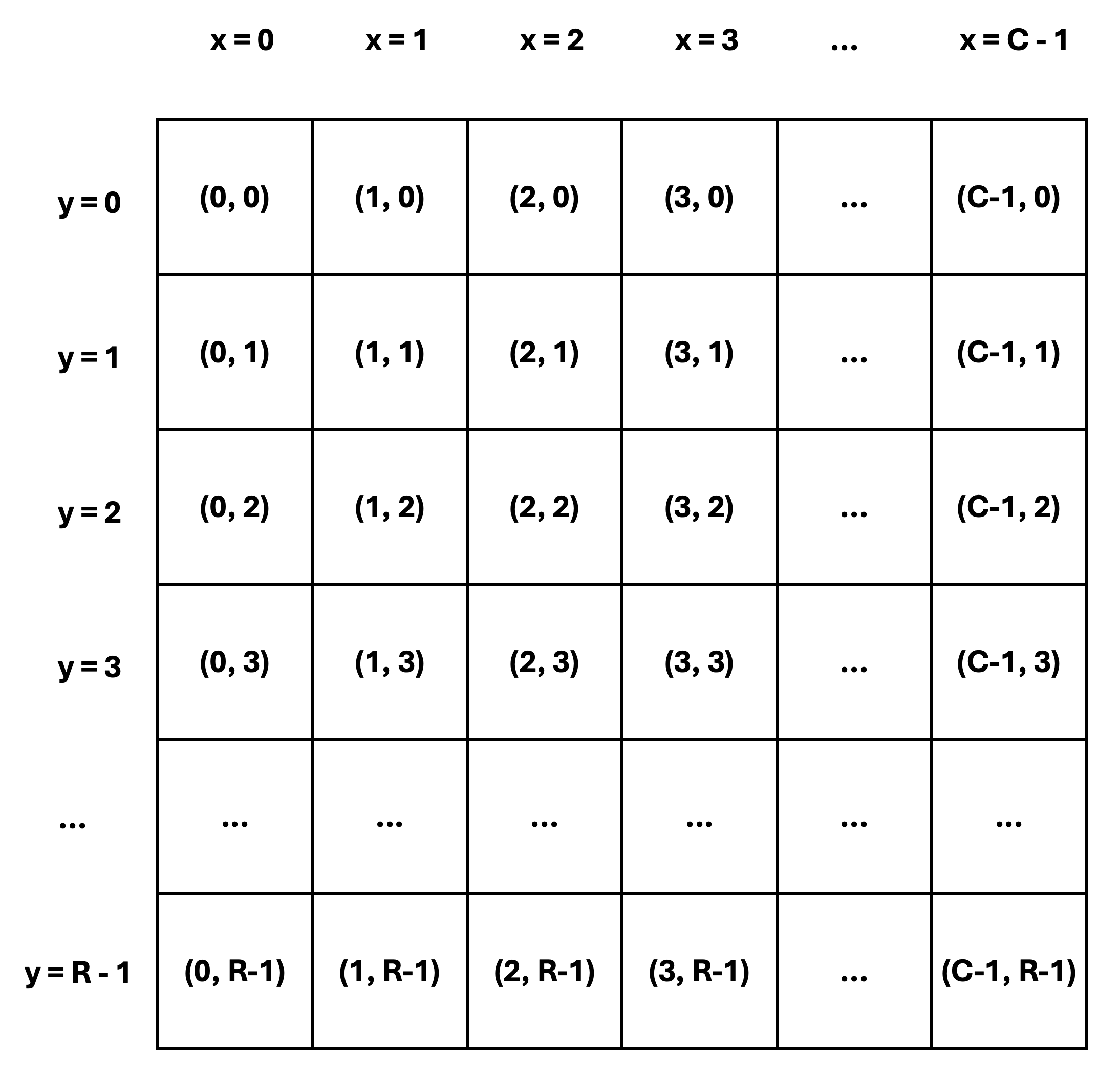
Figure 1: Tensix Core Grid

As shown in Figure 1, core coordinates use the x and y dimensions of the grid, rather than the row and column dimensions. As an example, core (1, 2) is the core in the third row and the second column, not the other way around.

x coordinates range from 0 to C - 1, where C is the number of grid columns. Similarly, y coordinates range from 0 to R - 1, where R is the number of grid rows. While the exact coordinates are not important in many cases, they are useful when examining logs and debug messages. They also become relevant when examining performance in more detail.

Determine Number of Available Tensix Cores

TT-Metalium provides a utility function compute_with_storage_grid_size() that returns the dimensions of the core grid as a CoreCoord object with elements x and y, representing the number of Tensix cores along the horizontal and vertical dimensions, respectively.

CoreCoord core_grid = device->compute_with_storage_grid_size();
uint32_t compute_cores = core_grid.x * core_grid.y;

Split Work Among Tensix Cores

Tenstorrent devices support multiple parallelization strategies. The grid structure of the Tensix processor enables various approaches to distributing work. In this lab, we will use a simple SPMD computational model similar to GPU programming to implement matrix multiplication on multiple cores. Each core will be responsible for producing approximately num_output_tiles/num_cores output tiles.

We will use a simple strategy of dividing the work as evenly as possible among the cores. We will also make a simplifying assumption that the matrix dimensions are divisible by the tile size. For example, if the matrix dimensions are 288x288 and the tile size is 32x32, then the number of output tiles is 9 * 9 = 81. Let us assume we choose to implement the matrix multiplication on 11 cores because other cores are needed for other tasks. Since 81 / 11 = 7.36, and the number of output tiles must be an integer, we choose 8 as the maximum number of output tiles per core. One way to divide the tiles is to assign the first four cores 8 output tiles each, and assign the remaining seven cores 7 output tiles each.

The diagram in Figure 2 shows how the output tiles are distributed among the cores. Each square represents a tile, and the color of the square corresponds to the core that is responsible for producing that tile.

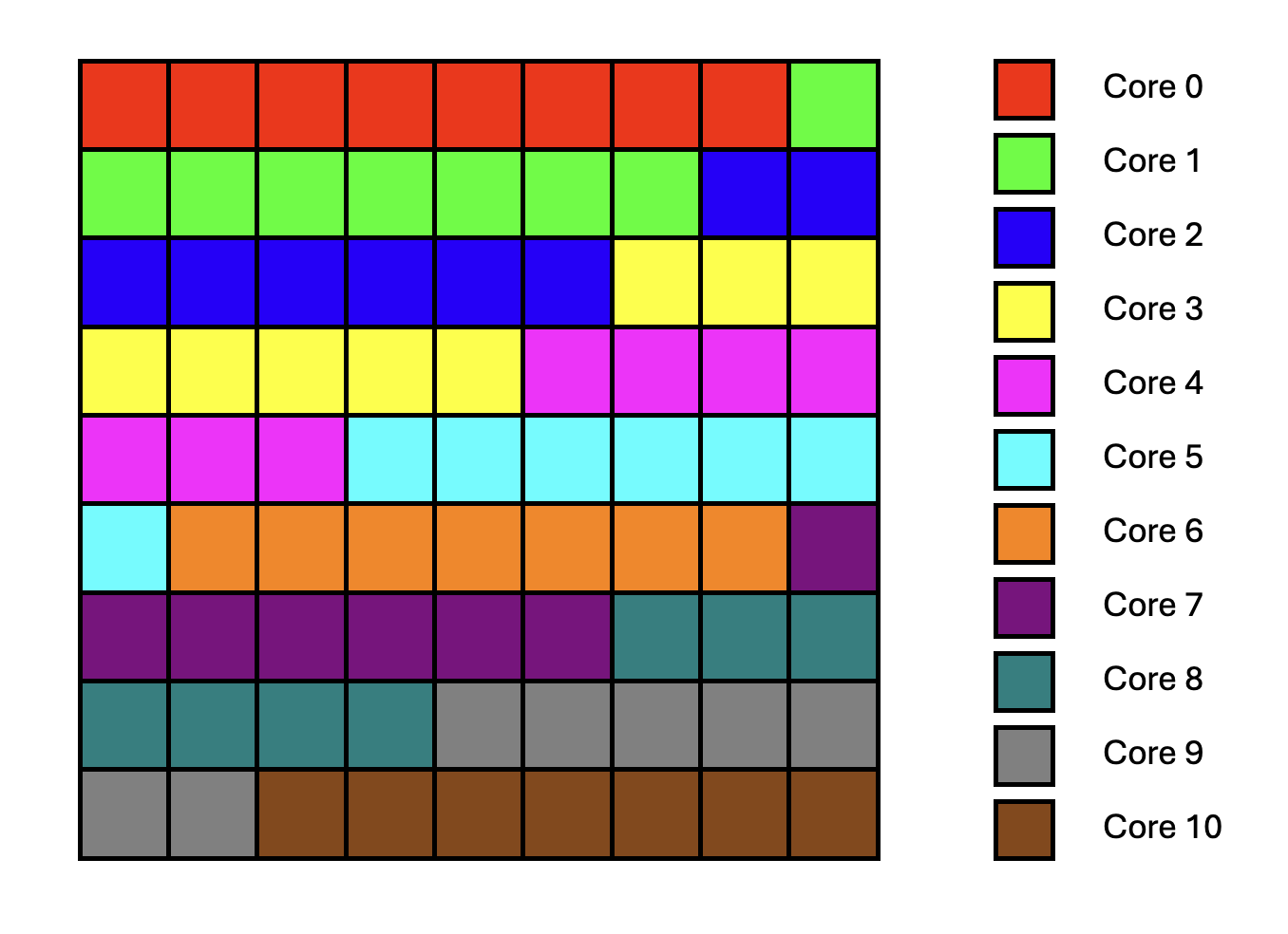
Figure 2: Output Tile Distribution on Multiple Cores

TT-Metalium includes utilities to simplify work distribution across cores. This is done in two steps:

1. Determine the amount of work each core should do.

2. Assign specific instances of work to specific cores, based on the amount of work each core should do, as determined in the first step.

TT-Metalium provides a utility function tt::tt_metal::split_work_to_cores(core_grid, work_units), which can be used to determine the amount of work each core should do. The function calculates how many work units each core should process, based on the total amount of work units and the number of available cores. The function distributes the work as evenly as possible, even if the number of work units does not divide evenly among the cores.

work_units is simply an integer that represents the total amount of work to be distributed. The meaning of work_units is determined by the specific problem being solved and the parallelization strategy being used. For example, for matrix multiplication, work_units could be any of the following:

• Number of elements in the output matrix. Since each output element can be computed in parallel, we could choose to assign individual elements to cores. While possible, this would be a poor choice when targeting Tenstorrent devices, since they can efficiently multiply whole tiles.

• Number of tiles in the output matrix. Similar to the above, we could choose to assign individual tiles to cores.

• Number of larger blocks in the output matrix. We could increase tile size, or use blocks of tiles in the output matrix as units of work to be assigned to cores.

If we assume that work units are the output tiles, the function may be called as follows:

#include <tt-metalium/work_split.hpp>

CoreCoord core_grid = device->compute_with_storage_grid_size();
uint32_t work_units = (M * N) / (TILE_HEIGHT * TILE_WIDTH);

auto [num_cores, all_cores, core_group_1, core_group_2, work_per_core_1, work_per_core_2] =
    tt::tt_metal::split_work_to_cores(core_grid, work_units);

The function returns a tuple containing several values:

• uint32_t num_cores: Number of cores used for the operation.

• CoreRangeSet all_cores: Set of all cores assigned to the operation.

• CoreRangeSet core_group_1: Primary group of cores, each handling work_per_core_1 amount of work.

• CoreRangeSet core_group_2: Secondary group of cores, each handling work_per_core_2 amount of work (empty if the work divides evenly).

• uint32_t work_per_core_1: Number of work units (e.g., output tiles) each core in the primary group processes.

• uint32_t work_per_core_2: Number of work units (e.g., output tiles) each core in the secondary group processes (0 if the work divides evenly).

The following properties describe the output of tt::tt_metal::split_work_to_cores:

• all_cores is the set of cores assigned work for this operation, containing exactly num_cores cores.

• If there are more cores in core_grid than the number of work units, all_cores may contain fewer cores than core_grid.

• all_cores is always the union of core_group_1 and core_group_2.

• The total amount of work work_units is always fully assigned: work_per_core_1 * core_group_1.num_cores() + work_per_core_2 * core_group_2.num_cores() == work_units.

• The function automatically handles uneven work distribution; there is no need to manage edge cases manually.

Given the earlier example of splitting 81 output tiles across a grid with 11 cores, split_work_to_cores may distribute the work as follows:

• num_cores = 11 (all cores are used)

• all_cores = Set containing coordinates of all 11 cores

• core_group_1 = A subset of four cores (each processing 8 tiles)

• core_group_2 = A subset of seven cores (each processing 7 tiles)

• work_per_core_1 = 8 (tiles per core in the primary group)

• work_per_core_2 = 7 (tiles per core in the secondary group)

A CoreRangeSet is a compact representation of an arbitrary set of logical cores, implemented as a collection of rectangular CoreRange objects. For example, all_cores contains every core that will do work, while core_group_1 and core_group_2 are disjoint subsets of those same cores. Rather than storing every core individually, each CoreRangeSet stores a vector of CoreRange objects.

Each CoreRange object is itself defined by two CoreCoord objects, start_coord and end_coord, each containing coordinates of the opposite corners of a rectangle of cores. The range includes all (x, y) cores where start_coord.x <= x <= end_coord.x and start_coord.y <= y <= end_coord.y. The CoreCoord class is just a pair of integer coordinates (x, y) identifying a single core on the device grid.

The CoreRangeSet class exposes a number of helpers, including:

• num_cores(): Returns the total number of logical cores covered by the CoreRangeSet.

• ranges(): Returns a const reference to a container of CoreRange objects to allow iterating over all CoreRange objects in the set.

• contains(CoreCoord): Returns true if and only if the given (x, y) core lies inside at least one of the CoreRange rectangles in the set, and false otherwise.

Finally, the CoreRange class provides an iterator interface to iterate over all CoreCoord objects in the range.

It is important to only create kernels on cores that have been assigned work (i.e., those in all_cores or core_group_*, and not over all cores in core_grid). Creating kernels on unused cores can cause undefined behavior or crashes if kernels are created but runtime arguments are not set on the core.

Create Circular Buffers and Kernels on Multiple Cores

Circular buffers (CBs) have to be created on each core participating in the computation. Each participating core will use its CBs to store the required tiles of matrices A, B, and C.

Each core can access only the CB instances created on that core; CBs are not shared across cores. Therefore, CB identifiers, such as CBIndex::c_0, don’t have to be unique across cores. In fact, it is common to use the same CB identifier for all cores running the same kernels, so that kernel code can be reused across cores. Given this, CBs can be created on all participating cores simply by passing all_cores (rather than a single core) to the function that creates circular buffers. Note that the create_cb helper function you used in Lab 1 needs to be updated to accept a CoreRangeSet of cores, which can then be passed on to the CreateCircularBuffer function. Alternatively, you could update create_cb to take a variant argument similar to the CreateCircularBuffer function, so it can accept either a single core or a set of cores.

Similarly, reader, compute, and writer kernels need to be created on all participating cores, which is also done by passing all_cores to the function that creates kernels.

Set Per-Core Runtime Arguments

The way to assign specific instances of work to specific cores is through runtime arguments for each kernel instance. We need to determine what arguments are needed for each kernel instance so that kernels on each core get sufficient information to perform only those operations that are needed for the output tiles assigned to that core. The reader and writer kernels need to generate correct tile indices into the underlying tensors, while the compute kernel needs to loop over the correct number of output tiles and inner dimension tiles.

All kernel arguments that need to be different between cores must be passed as runtime arguments and set differently for each core. This is because their values will be known only at runtime, when the work distribution is known. Arguments that are the same for all cores and are known at compile time can be passed as either compile-time arguments or runtime arguments. As discussed in Lab 1, choosing compile-time vs. runtime arguments trades off potential performance gains from compile-time constants against the cost of recompiling kernels for each different set of argument values.

To set core-specific runtime arguments, you will need to iterate over all core ranges in core_group_1 and then iterate over all cores in the range and set the runtime arguments for each core. Similarly, you should also iterate over all core ranges in core_group_2 to set core-specific runtime arguments corresponding to the amount of work for the secondary group of cores.

Inspecting and Choosing Cores

As shown earlier, the number of available compute cores on the device can be obtained using the compute_with_storage_grid_size() TT-Metalium C++ API. To call this API, you need to get the device object, which can be obtained from the program state object (i.e., prog_state.mesh_device.get()).

In this lab, you will run matrix multiplication with a varying number of cores. The number of cores actually used is entirely controlled by which cores you include in your core sets when creating circular buffers and kernels. Any cores without kernels created on them will remain idle for that program (in real applications, they would be allocated to other tasks).

To use all available compute cores, you can pass the full available compute grid to the work-splitting helper, obtain all_cores, and then create CBs and kernels on all cores in all_cores, passing appropriate runtime arguments to the kernels. To use fewer cores, you can modify the core grid to select only a subset of cores simply by modifying the x and y dimensions of the core grid before passing it to the work-splitting helper. The rest of the code can usually remain the same, because the work-splitting helper automatically distributes the work evenly among the smaller set of cores. As a result, the same total number of output tiles ends up spread across this reduced set of cores, with each tile still computed exactly once. It is important to remember that every core on which you create a kernel must also receive appropriate runtime arguments for that kernel. Creating a kernel on a core without setting runtime arguments can lead to undefined behavior, including crashes or hangs.

Exercise 1: Multi Core Matrix Multiplication

In this exercise, you will implement matrix multiplication on multiple Tensix cores by modifying your Lab 1 solution.

Perform the following steps:

1. Create a new program for multi core matrix multiplication by copying your Lab 1 solution for single core matrix multiplication in TT-Metalium, then extend it to distribute work across multiple cores, as described in the following steps.

2. Make the core grid used for computation parameterizable and add assertions to ensure the specified core grid size is valid (i.e., not outside the boundaries of the available compute grid). Then use the split_work_to_cores function to determine the number of output tiles each core should compute, as described in the previous sections.

3. Create CBs on all cores participating in the computation, and create reader, compute, and writer kernels on all participating cores, as described in the previous sections.

4. Set core-specific runtime arguments for the reader, compute, and writer kernels so that kernels on each core perform the operations appropriate for the subset of output tiles assigned to that core.

5. Update the reader kernel to read the subset of input tiles required for the subset of output tiles assigned to a given core, based on the parameters passed to the kernel as runtime arguments. Similarly, update the writer kernel to write the subset of output tiles assigned to a given core, based on the runtime arguments. Finally, update the compute kernel to compute results for the appropriate number of output tiles, based on the runtime arguments.

6. Verify correctness by comparing the results against the reference matrix multiplication you created in Exercise 1 of Lab 1.

7. Run the multi core implementation using:

   • Work distributed over a 5x5 core grid

   • Work distributed over a 10x10 core grid

   • Work distributed over all available compute cores.

8. Profile and compare the performance of the three runs using the device profiler introduced in Lab 1. Ensure that you build with the Release option and that DPRINTs are disabled.

9. Create a plot showing the relationship between speedup and the number of cores used. The speedup should be expressed relative to the performance of the single core implementation from Lab 1.

Important Note

If you are working on a device with fewer than 100 Tensix cores, adjust the core grid sizes accordingly.

Data Reuse in Multi Core Matrix Multiplication

Motivation

In the basic multi core implementation, each core computes one output tile at a time. For each output tile C[i,j], the reader kernel fetches all tiles along the inner dimension K for both the corresponding row of A and column of B. This is inefficient because tiles from the input matrices are fetched from DRAM multiple times.

Consider a concrete example with matrices A and B of shape 4x4 tiles, producing the resulting matrix C of shape 4x4 tiles. To compute output tiles C[0,0] and C[0,1]:

Output Tile	Tiles Read from A	Tiles Read from B
C[0,0]	A[0,0], A[0,1], A[0,2], A[0,3]	B[0,0], B[1,0], B[2,0], B[3,0]
C[0,1]	A[0,0], A[0,1], A[0,2], A[0,3]	B[0,1], B[1,1], B[2,1], B[3,1]

Notice that the entire row 0 of A is read twice; once for C[0,0] and once for C[0,1]. In general, for an MxK matrix multiplied by a KxN matrix, producing MxN output tiles:

• Each row of A is read N times (once per column of C in that row)

• Each column of B is read M times (once per row of C in that column)

This redundant DRAM traffic can become the performance bottleneck, especially as matrix dimensions grow. A simple optimization would be to store the whole row of A in a temporary on-chip SRAM, and then use it to compute all the output tiles in the row. However, this simple approach doesn’t scale well to large matrices because the amount of available on-chip memory may not be sufficient to hold the entire row of A. Also, this approach only reuses data in rows of A, but not in columns of B.

Blocked Matrix Multiplication

Instead of considering one row at a time, a more general approach is to group output tiles into rectangular blocks and assign such rectangular blocks to cores. For example, consider Core 1 in Figure 2, discussed earlier. Core 1 needs the first row of A and the last column of B to compute the output tile in the top right corner of the output, and only for that tile. Therefore, this data cannot be reused for any other computation. If we distribute work across e.g., 9 cores instead, such that each core computes 3x3 output tiles, then each core can use a row of A to produce output of three tiles in the same row of the output. Similarly, each core can use a column of B to produce output of three tiles in the same column of the output. This is shown in Figure 3.

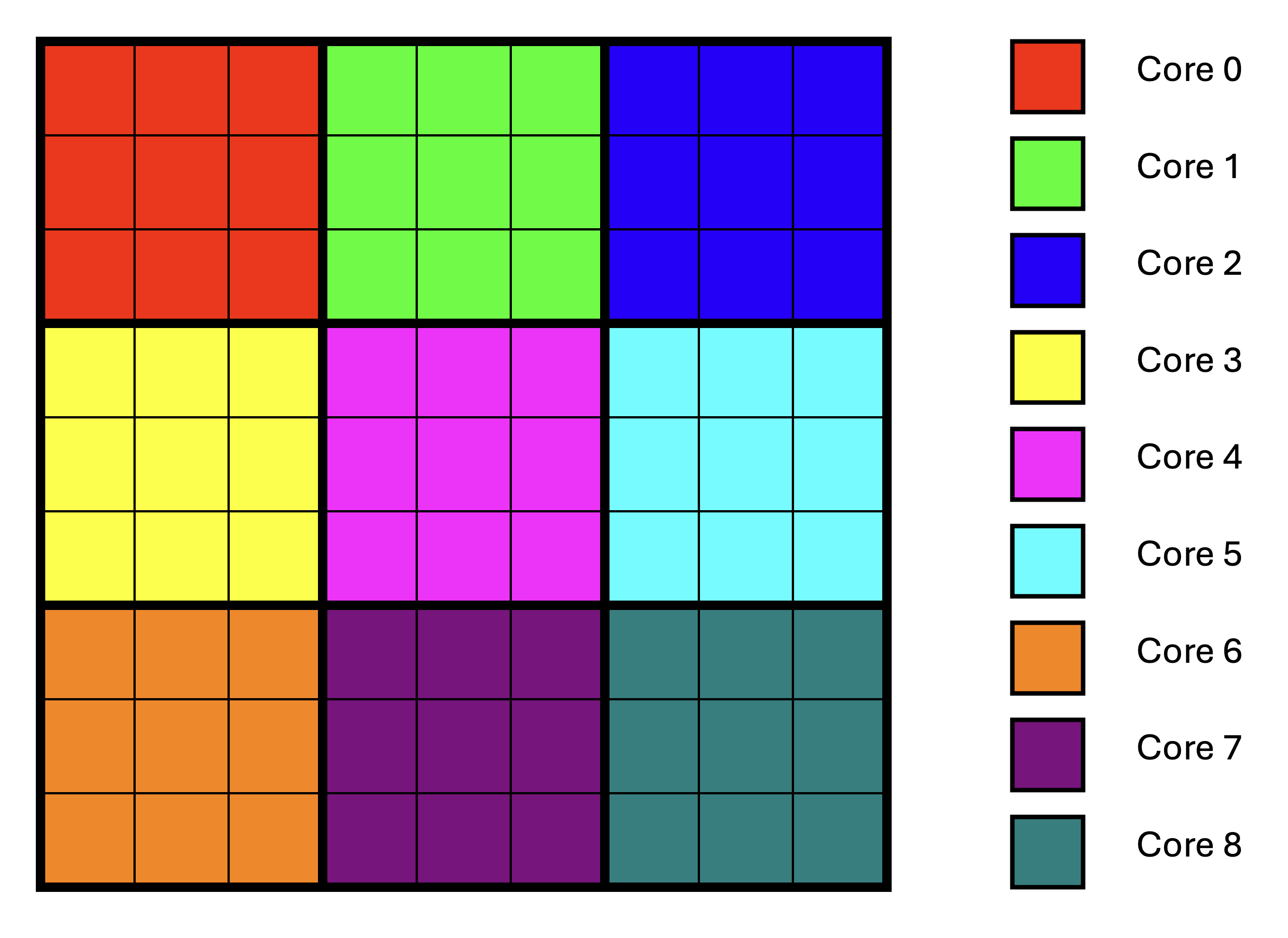
Figure 3: Output Tile Distribution on Multiple Cores Using Blocking

Observe that there is no data reuse across cores; each core still needs to read input data for its own block of output tiles, some of which is the same as the data read by other cores. Also observe that this approach requires the number of tiles to be a multiple of the number of cores in each dimension of the core grid to ensure that blocks of tiles are rectangular, thus maximizing data reuse.

Comparing Figure 3 to Figure 2, we went from using 11 cores to using 9 cores. As a result, the maximum number of tiles per core increased from 8 to 9. While this increases the amount of computation each core performs, it can still provide a net performance benefit when the program is memory-bound, because the performance gain from data reuse may outweigh the performance loss from having fewer compute cores. Alternatively, we could pad the matrix dimensions to make them a multiple of the number of cores in each dimension.

If the program is compute-bound, we may choose to:

• Not use blocking if a lower number of cores causes performance degradation because data reuse is not beneficial.

• Add more cores across one or both dimensions of the core grid, if a higher number of cores is available and will divide the number of tiles evenly.

Limiting On-Chip Memory Usage

Assigning rectangular blocks of output tiles to cores doesn’t address the problem that bringing, for example, an entire row of A into on-chip SRAM may not be possible due to limited on-chip memory. In fact, for data reuse to be fully effective with blocking, we need multiple rows of input tiles in on-chip memory at the same time. The solution is to break down the K dimension into smaller chunks of tiles and compute partial results for each chunk, which require only a subset of the input tiles that is small enough to fit in on-chip SRAM. Since partial results eventually need to be accumulated, they should also be stored in on-chip SRAM to avoid performance degradation due to repeated accesses to off-chip DRAM.

We will again assume multiplication of two matrices A of shape MxK and B of shape KxN, with the resulting matrix C having shape MxN. We will assume that all the matrix dimensions are divisible by the tile size, and use the notation:

• Mt = M / TILE_HEIGHT

• Nt = N / TILE_WIDTH

• Kt = K / TILE_WIDTH

to denote the number of tiles in the M, N, and K dimensions, respectively.

In blocked matrix multiplication, each core is responsible for computing a rectangular block of output tiles C_block consisting of

• M_block_tiles rows of tiles, and

• N_block_tiles columns of tiles.

The division of the Mt and Nt dimensions into blocks is done simply by dividing the number of tiles in each dimension by the number of cores in that dimension of the core grid.

To compute all tiles in C_block, the core needs the matching tiles from A and B:

• The tiles of A covering all rows of this block and the full K range:

  • M_block_tiles x Kt block of tiles (call this A_block)

• The tiles of B covering the full K range and all columns of this block:

  • Kt x N_block_tiles block of tiles (call this B_block).

Taken together, A_block and B_block are typically too large to fit in on-chip SRAM. To fix this, we split the Kt dimension into smaller K-blocks of size K_block_tiles, such that num_k_blocks = Kt / K_block_tiles. For each K-block index b in range 0 .. num_k_blocks - 1 we define:

• A_slab(b): tiles of A, not consisting of full rows, but rather of only appropriate K_block_tiles tiles in the row (size: M_block_tiles * K_block_tiles).

• B_slab(b): tiles of B, not consisting of full columns, but rather of only appropriate K_block_tiles tiles in the column (size: K_block_tiles * N_block_tiles).

If we choose K_block_tiles carefully, then both A_slab(b) and B_slab(b), and the partial results for C_block can all fit into the on-chip SRAM at the same time.

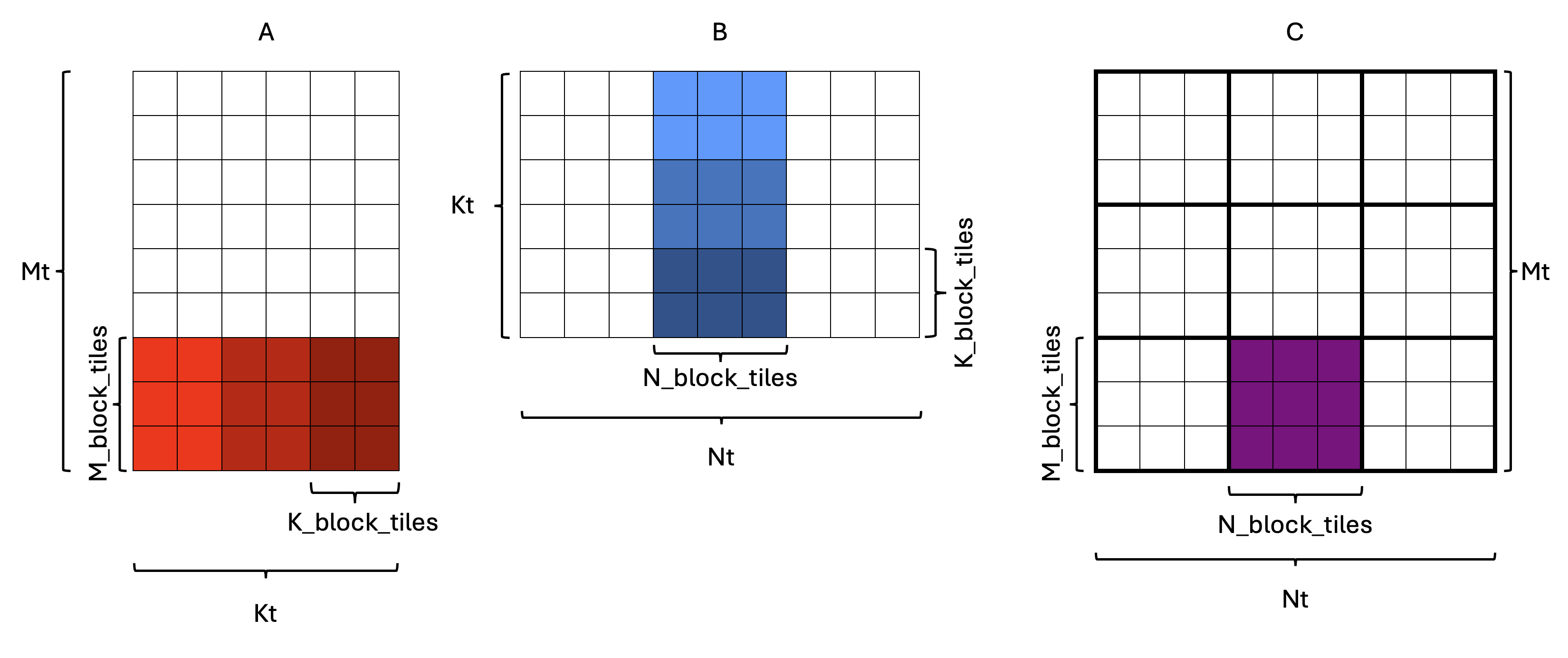
Figure 4: Splitting the Kt dimension into K-blocks

An example is shown in Figure 4, where each rectangle represents a tile. In this example, Mt = 9, Nt = 9, Kt = 6, with the core grid size being 3x3. As a result, M_block_tiles = 3 and N_block_tiles = 3, which means C_block has shape 3x3. One of the C_block tiles is highlighted in purple in the output matrix C. The corresponding A_block and B_block tiles are highlighted in shades of red and blue in the input matrices A and B, respectively. If we assume that A_block and B_block are too large to fit in on-chip SRAM, we split the Kt dimension into K_block_tiles = 2, which means there are num_k_blocks = 3 K-blocks. Therefore:

• A_slab(b) has shape 3x2 tiles, and

• B_slab(b) has shape 2x3 tiles.

Each “slab” is indicated by a different shade of its respective color in Figure 4.

To see what computation needs to be performed such that each slab is read only once, consider the computation for a single output tile C[i][j] within C_block:

We can split the sum over k into consecutive chunks corresponding to K-blocks. Each K-block b spans some range of k values: (b * K_block_tiles) .. ((b + 1) * K_block_tiles - 1). Given this, we can decompose the computation of C[i][j] as follows:

Decomposing the original equation across K-blocks, we get:

Define the partial result for block b as:

A key observation is that the partial result equation needs only tiles from the current K-block b to compute the partial result for C[i][j](b), which is exactly what A_slab(b) and B_slab(b) contain. Considering the example in Figure 4, this means that only the slabs with the same shading of their respective color (e.g. lightest blue and lightest red) need to be in on-chip SRAM at the same time. This makes intuitive sense, since matrix multiplication involves multiplying elements with matching K indices.

To get the final result, we need to add partial results for all K-blocks:

Observe that the above equations concern only a single tile of the output C[i][j]. This computation needs to be done for all tiles in C_block, i.e., for all i and j in 0 .. M_block_tiles - 1 and 0 .. N_block_tiles - 1. If we did this naively, we would iterate over i and j in the outer loops and then compute the partial result for each tile, which would not be conducive to data reuse. Instead, we need to iterate over K-blocks in the outer loop, bring A_slab(b) and B_slab(b) into on-chip SRAM, and then compute the contribution of this K-block to all C[i][j] tiles in C_block. Given that matrix multiplication is a linear transformation, such loop interchange does not change the result (ignoring floating-point considerations), as discussed in Lab 1.

Note that if understanding the above equations with respect to tiles is confusing, try thinking of them as individual elements rather than tiles. The underlying math is the same, but it becomes easier to verify your understanding.

Blocked Matrix Multiplication with Data Reuse Pseudocode

The overall approach can be summarized by the following pseudocode for a compute core:

// For every K-block:
for (b in 0 .. num_k_blocks - 1) {
    Ensure that A_slab(b) is in CB0 // Size: M_block_tiles * K_block_tiles.
    Ensure that B_slab(b) is in CB1 // Size: K_block_tiles * N_block_tiles.
    // For every output tile (i,j) in this C_block:
    for (i in 0 .. M_block_tiles - 1) { // For every row in C_block
        for (j in 0 .. N_block_tiles - 1) { // For every column in C_block
            // Get the current accumulator tile for C(i,j)
            acc_tile = zero_tile()
            if (b != 0) {
               // Middle or last K-block: partial result for C(i, j) already exists.
               // Load the partial result built so far
               acc_tile = partial_C_tile(i, j)
            }

            // Compute partial result for block b and add it to acc_tile
            for (k_local in 0 .. K_block_tiles - 1) { // Iterate over K dimension of the K-block
                // Indices into the current A and B slabs
                a_tile = A_slab_tile(i, k_local)
                b_tile = B_slab_tile(k_local, j)

                // Multiply and accumulate into the accumulator tile
                acc_tile += matmul(a_tile, b_tile)
            }

            // Store updated result for C(i,j)
            if (b == num_k_blocks - 1) {
               // Last K-block: acc_tile has the final result for C(i,j)
               // Store it to the final destination.
               final_C_tile(i, j) = acc_tile
            } else {
               // Not last K-block: acc_tile is a partial result to be reused later
               partial_C_tile(i, j) = acc_tile
            }
        }
    }
}

Data Reuse Evaluation

Consider the example in Figure 4, where Mt = 9, Nt = 9, Kt = 6, and the core grid is 3x3. With the basic (non-blocked) approach, each core computes one output tile at a time. For each output tile C[i][j], the core reads the full corresponding row of tiles of A and the full corresponding column of tiles of B from DRAM.

For each output tile C[i][j] we need Kt = 6 tiles from A and Kt = 6 tiles from B. Given that the basic multi core approach doesn’t involve any reuse, such reads are repeated for every one of the Mt * Nt = 81 output tiles in C, resulting in Mt * Nt * 2 * Kt = 81 * 2 * 6 = 972 tile reads.

With the blocking strategy and K-blocking described earlier, the core computes an entire 3x3 C_block at a time and splits the inner dimension into K-blocks. For any given core, every tile of A and B that it needs for its own C_block will be read exactly once. Since each core computes only the output tiles in its own C_block, it needs to read only M_block_tiles * Kt tiles from A and Kt * N_block_tiles tiles from B, which for this example means 18 tiles from A and 18 tiles from B. Each of the num_cores = 9 cores reads this many tiles, for a total of num_cores * (M_block_tiles * Kt + Kt * N_block_tiles) = 9 * (3 * 6 + 6 * 3) = 324 tile reads.

Thus the blocking strategy reduces the total number of tile reads by a factor of 3 for this example. Such a reduction can produce significant performance improvements when the operation is memory-bound.

Blocked Matrix Multiplication in TT-Metalium

Most of the code needed for blocked matrix multiplication is similar to the basic multi core implementation from Exercise 1. The key new addition is the introduction of an intermediate circular buffer (CB) to hold partial results. As discussed in Lab 1, kernels can read from and write to the same CB, allowing the CB to be used as temporary storage for partial results. Since CBs behave as FIFO queues, they are not typically used as raw memory storage. Instead, they are used as a stream of tiles that carry partial results between phases of the computation. In the context of blocked matrix multiplication, this results in the following pattern:

• The compute kernel produces a block of partial results into an intermediate CB using cb_reserve_back, pack_tile and cb_push_back.

• On the next K-block, the same compute kernel reloads these partial results from the CB so it can accumulate the next K-block’s contributions. It calls cb_wait_front to ensure the previous partial results are available, reads them and uses cb_pop_front to indicate they have been consumed.

• The kernel computes another K-block’s contributions and adds them to the partial results.

• If this is not the last K-block, write the updated partial results back to the intermediate CB (again via reserve_back / pack_tile / push_back) to be used in the next iteration.

• If this is the last K-block, write the fully accumulated tiles into a separate output CB (also via reserve_back / pack_tile / push_back), for the writer kernel to consume.

As can be seen, the CB holding partial results is not treated as a raw memory array; it is still a FIFO queue. What changes is who consumes and produces that queue over time: the compute kernel both produces and later consumes tiles from the same CB, using the standard reserve/push/wait/pop protocol to keep the streaming semantics, while treating the tiles themselves as partial sums rather than final outputs.

Exercise 2: Multi Core Matrix Multiplication with Data Reuse

In this exercise, you will implement a blocked multi core matrix multiplication with data reuse on the device, based on the blocking and intermediate CB ideas described above. You will compare performance to the multi core implementation with equivalent core grid sizes from Exercise 1.

Follow these steps to complete the exercise:

1. Create a new program for data reuse by copying your multi core matrix multiplication program from Exercise 1, then extend it to add blocking variables and an intermediate CB, as described in the following steps. Make sure matrix and tile sizes are parameterizable and set to the same values as in previous exercises: A: 640x320, and B: 320x640. Use predefined variables TILE_HEIGHT and TILE_WIDTH to compute the number of tiles. As before, you can assume that TILE_HEIGHT == TILE_WIDTH, and that M, N, and K are divisible by TILE_HEIGHT.

2. Add a parameter for K_block_tiles. This parameter needs to be chosen so it divides Kt evenly. A lower value of K_block_tiles allows for larger matrix sizes to fit into the available on-chip SRAM, since lower K_block_tiles means fewer tiles in each slab. A higher value increases on-chip SRAM usage, but results in fewer iterations of the outer loop over K-blocks, which means that partial results, whose size does not depend on K_block_tiles, are loaded from and stored into CBs fewer times.

   The tile size is 32x32 on all Tenstorrent architectures, as of the time of this writing. Given the matrix sizes above, the number of tiles in the K dimension is Kt = 320 / 32 = 10. Given this, valid values for K_block_tiles are 1, 2, 5, or 10. The impact of this parameter on performance is often small, particularly for small matrix sizes, and may be overwhelmed by other factors. Set K_block_tiles to 2 to demonstrate that your code works with a non-trivial value of this parameter.

   Note: Should the tile size be different on the architecture you are working with, the value of K_block_tiles may need to be adjusted accordingly. To be on the safe side, add an assertion to check that K_block_tiles divides Kt evenly.

3. Make the core grid used for computation parameterizable, then determine appropriate values for the other blocking variables, based on the core grid size and the matrix sizes. Also assume that the number of tiles divides evenly into the number of cores in the corresponding dimension.

4. Size circular buffers based on the blocking variables, keeping in mind the following:

   • Input CBs need to store full A_slab and B_slab and should use double buffering.

   • Output CB needs to store the full C_block, and should not use double buffering. Since each core computes a whole C_block, there is no need to double buffer.

   • Intermediate CB needs to store the partial results, whose size is the same as a full C_block. Since the same kernel will both produce and consume the partial results, double buffering would not provide any benefit.

   • Create CBs on all cores participating in the computation. Since in this exercise it is not necessary to use the split_work_to_cores function, you can construct the set of all cores from the core grid dimensions, as follows:

     CoreRangeSet all_cores{CoreRange(CoreCoord(0, 0), CoreCoord(core_grid.x - 1, core_grid.y - 1))};
     

5. Modify reader and writer kernels to read and write the appropriate tiles from the circular buffers. The reader kernel should read the appropriate tiles (A_slab(b) and B_slab(b)) from the circular buffers in the same order that the compute kernel will use them. Order tiles within each slab in the CB in row-major order. The writer kernel should read the C_block tiles from the output circular buffer in row-major order and write them to the output tensor in appropriate locations.

6. Modify the compute kernel to use the intermediate buffer to reload and update partial results.

   • When you call mm_init, one of the arguments is the output circular buffer index. Given that matrix multiplication results will be written into either the output or intermediate buffers, you can use either of the two circular buffer indices in a call to mm_init. This is because mm_init uses the output circular buffer index only to determine output data format related parameters, which are the same for both the output and intermediate CBs.

   • An efficient way to accumulate partial results is to use the destination register array. Recall that the matmul_tiles function adds to the existing values in the destination register rather than overwriting existing content. Therefore, if a partial sum is first loaded into the destination register, matmul_tiles will also accumulate the result into the destination register in one operation.

   • Storing partial results into the intermediate CB is done in the same manner as storing the final results into the output buffer. However, loading data from the intermediate buffer into the destination register requires a new operation:

     • copy_tile(in_cb_id, in_tile_index, dst_tile_index) defined in tt_metal/hw/inc/api/compute/tile_move_copy.h copies a tile from the intermediate CB to the destination register array at the specified index.

     • Before calling this function, you need to call copy_tile_to_dst_init_short(in_cb_id) to set up the Tensix Engine for the copy operation.

     • Since the compute kernel code will alternate between copying data and multiplying tiles, after the copy operation completes, we need to call mm_init_short(in0_cb_id, in1_cb_id) to set up the Tensix Engine for multiplication again. Observe that we are calling _short versions of the initialization functions (both mm_init_short and copy_tile_to_dst_init_short), which are faster than the “full” versions. The first call to mm_init performs more initialization steps that are no longer needed in subsequent calls, and these operations are common to both the copy and multiplication operations, which is why the _short versions are sufficient for later calls.

     • For optimal performance, make sure to call these initialization functions only when required.

   • Remember that an efficient way to initialize all the tiles in the destination register array to 0 is to call tile_regs_acquire.

   • Remember that tile_regs_acquire does more than just set the destination register array to 0. As such, it must always be called before using the destination register. Specifically, it must be called before calling copy_tile, but does not need to be called between a call to copy_tile and a call to matmul_tiles (doing so would be destructive, because it would overwrite the data that was just copied into the destination register array).

   • When writing to or reading from the intermediate CBs, you could wait/reserve the number of tiles for the whole block of partial results at once. However, a simpler option is to just push and pop one tile at a time. This is possible because the i, j loop nest iterates over indices in the same order for every block.

     Don’t forget to call cb_pop_front for the intermediate CB at the appropriate time to free up space for the next iteration.

   • Similar reasoning applies to the output circular buffer. However, given that the output CB is written by the compute kernel and read by the writer kernel, it is better for the compute kernel to push one tile at a time to allow the writer kernel to start writing the results as soon as they are available.

   • When writing the final results for the C_block tiles into the output CB, write the tiles in row-major order, as the writer kernel expects.

7. Modify the code that sets runtime arguments to pass appropriate parameters for the kernels on each core. Note that in this case it is not required to use the split_work_to_cores function, because we are making a simplifying assumption that the number of tiles divides evenly into the number of cores in the appropriate dimension. You can simply iterate over the x and y dimensions of the core grid, construct CoreCoord for each coordinate and set the runtime arguments for the corresponding core.

8. Run your data reuse implementation and compare the output tensor to the reference implementation to ensure that the results are correct.

9. Finally, profile your data reuse implementation using the device profiler for the following cases:

   • 5x5 core grid

   • 10x10 core grid

   Compare the firmware time of the data reuse implementation against the basic multi core implementation with equivalent core grid sizes from Exercise 1.

10. Create a plot showing the relationship between speedup and the number of cores used. The speedup should be expressed relative to the performance of the single core implementation from Lab 1. Compare this plot to the one from Exercise 1.

Important Note

If you are working on a device with fewer than 100 Tensix cores, adjust the core grid sizes and/or matrix sizes accordingly to ensure that the number of tiles divides evenly into the number of cores in the appropriate dimension.

Potential Additional Optimizations

In this lab, you explored basic optimizations to implement data reuse in a multi core matrix multiplication program. There are many other ways in which the code could be further optimized. Here we list some examples:

1. Use Multiple Destination Registers in the Destination Register Array As discussed in Lab 1, the destination register array in the Tensix core can hold multiple tiles of data. So far, we have only used a single tile in the destination register array, but the TT-Metalium programming model exposes the array capable of holding up to eight tiles of data. We could leverage this extra storage to keep multiple output tiles active at once. By doing this, we could amortize the cost of setting up the Tensix Engine for multiplication and reduce how often data is packed into CBs. Conceptually, instead of computing a single output tile, packing it, and then moving on to the next, we compute a small rectangular patch (up to eight tiles) of the output in one shot while the corresponding input tiles are already in CB. Once that patch is fully accumulated in the destination registers, we pack all of its tiles out together in a batch. This better matches the hardware’s vectorization and register file structure and typically provides a throughput improvement.

2. Subblocking the Output On top of using multiple destination registers, we could go further by introducing subblocking: instead of treating everything a core is responsible for as one big output region, we break that region into smaller rectangular patches. The main motivation for this is reduction in on-chip memory usage. A smaller patch means fewer output tiles need to live in registers at once and fewer partial results need to be stored in the intermediate CB. That makes it easier to keep the active data set within on-chip memory limits, allowing more aggressive blocking along the inner dimension, and often enables larger overall matrix sizes without exceeding on-chip memory limits.

   Mechanically, subblocking just adds one more level of tiling around the loops you already have. Rather than sweeping the entire per-core output area in a single nested loop, we first step over patches, and inside each patch we iterate over its local tile coordinates. For each patch we reload its partial results into the destination registers, run the inner dimension accumulation for that patch, and then store updated results back to the appropriate buffer. The overall pattern of blocking along the inner dimension, using an intermediate CB for partial results, and exploiting multiple destination registers stays the same. Subblocking simply applies it to a smaller output region at a time so the live data footprint is more tightly controlled.

3. Sharing Memory for Output and Intermediate CBs Given that the amount of on-chip SRAM is limited, TT-Metalium CBs support sharing the same memory region for multiple CBs. We can exploit this by observing that partial results and output results are never “live” at the same time; we always finish consuming one before we start writing to the other. Dedicating a separate region for partial results means less room for inputs or larger tiles.

   In practice, sharing memory between the output and intermediate CBs can be achieved by configuring a single circular buffer allocation and exposing it through two logical views (two different CB indices) that point into the same physical memory. The compute kernel then enforces a strict ordering: wait for all tiles in a given range to be written out, reuse that range as intermediate storage for partials, and only after those partials are fully consumed reuse it again for final output.

4. Batching Tile Reads and Writes Another possible optimization is to read multiple tiles that are contiguous in memory, instead of one tile at a time. In the exercises so far, each tile for A or B is fetched with its own DRAM read, which is simple but involves multiple transfers, which may result in larger per-read overhead. Because the matrices are stored in a tiled layout, with tiles stored in row-major order, the tiles needed for a contiguous segment of a row are also contiguous in memory. That means a core could reserve space for multiple tiles (e.g., an entire row slice of a K-block) in its circular buffer and then read all those tiles at once, reducing the number of DRAM transactions, which usually improves effective bandwidth, and lowers the per-tile cost of getting data into on-chip SRAM.

Conclusion

In this lab, you extended your understanding of matrix multiplication on Tenstorrent devices beyond a single core. You saw how:

• The same reader-compute-writer kernel structure from Lab 1 can be reused in a multi core setting by carefully distributing output tiles among cores.

• TT-Metalium’s static parallelism model requires you to explicitly choose which cores participate and how many tiles each core processes, and to ensure that every core with kernels also receives runtime arguments derived from tensor metadata.

• Introducing data reuse through blocking and intermediate CBs allows partial results to remain on-chip across multiple passes over the inner dimension, reducing traffic to device memory and often improving performance.

The concepts introduced here, multi core work distribution and data reuse, are fundamental when scaling workloads on Tenstorrent devices. They also provide a foundation for more advanced topics.